When dealing with noisy data, many of us reach for the same tool first: a moving average. It is one line of code, it is intuitive, and it does remove noise. The catch is that it tends to do a bit more than that. A moving average is a fairly blunt instrument: alongside the jitter, it also tends to soften structure — flattening peaks, filling in troughs, and smearing the shape of the features we may actually care about. If all we want is a calmer-looking line, for example to visualize trends over a long period, that is usually fine. If we care about how tall a peak is, how wide a response is, or how fast something is changing, a plain average can quietly discard the part we wanted.
The Savitzky-Golay filter keeps more of it, using one simple idea — fit a small polynomial to a sliding window instead of averaging it. While this filter won’t save any lag, it provides a feature that makes it worth knowing: it hands us a smoothed derivative almost for free. It can also find applications in finance, where the moving average and its exponential cousin are the defaults.
All the plots below come from a small, reproducible script (synthetic data, fixed seed); the snippets in the text are the load-bearing parts of it.
The problem: a moving average smears structure
Here is a sharp peak buried in noise. We smooth it two ways with the same 41-point window: a centred moving average, and Savitzky-Golay.
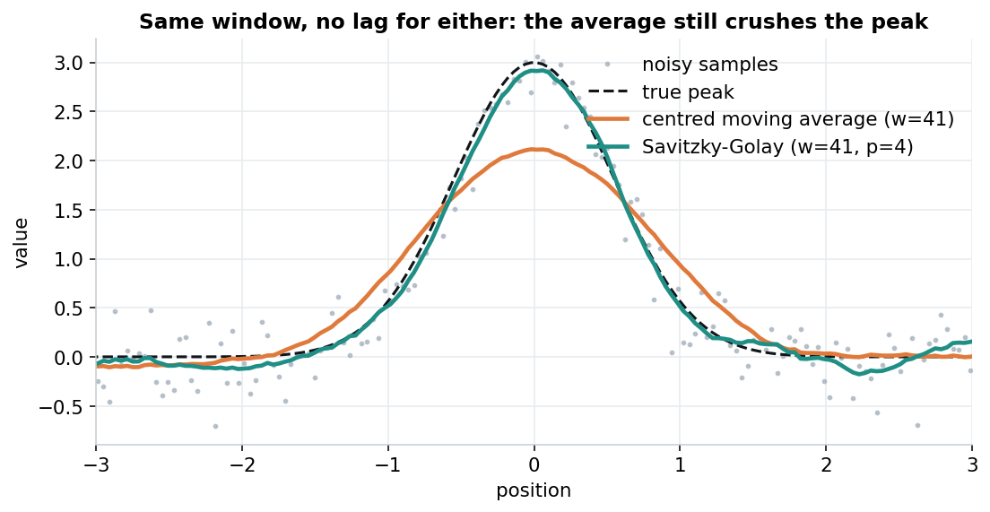
Same window, neither filter shifted in time: the moving average still pulls the peak down toward its neighbours, while Savitzky-Golay fits the curvature and keeps more of the height.
The true peak height is 3.0. The moving average reports about 2.1 — roughly a 30% shortfall — because averaging a peak together with its lower neighbours tends to pull it down. Savitzky-Golay stays much closer to the truth.
This is not a timing artefact. Both filters here are centred, so neither is shifted left or right (more on that below). The moving average loses the peak mainly because averaging assumes the data is locally flat, and a peak is about as far from flat as it gets. The same effect can quietly distort widths, areas, and other shape information we might be relying on.
Core idea
Instead of averaging the window, Savitzky-Golay fits a low-order polynomial to it by least squares, and takes the value of that polynomial at the centre of the window. Then it slides the window over by one and repeats.
That is most of the idea. A moving average implicitly assumes the signal inside the window is flat — a degree-0 fit, whose best constant is the mean. Savitzky-Golay lets it be a gentle curve (degree 2, 3, 4…). Real signals near a peak or a turn are usually curved rather than flat, so the polynomial fit tends to follow them instead of cutting the corner.
There is a neat practical consequence: because a least-squares polynomial fit is a linear operation, for a fixed window and order it collapses to a fixed set of weights. So Savitzky-Golay ends up being just a convolution — one cheap pass over the data, O(n × window). We get the curvature-awareness of a per-window fit at the price of a single dot product per point, and the weights only need computing once.
Usage: The SciPy version
SciPy ships it as scipy.signal.savgol_filter, so smoothing is a one-liner:
import numpy as np
from scipy.signal import savgol_filter

x = np.linspace(-6, 6, 300)
y_true = 3.0 * np.exp(-(x ** 2) / 0.6)            # a sharp peak
noisy = y_true + np.random.default_rng(7).normal(0, 0.25, x.size)

smooth = savgol_filter(noisy, window_length=41, polyorder=4)
Two parameters, no state to manage, nothing beyond SciPy.
Two knobs
There are two things to tune, and they pull in opposite directions:
- Window length (must be odd): how many points each poly-fit sees. Bigger = smoother, but it starts to distort features narrower than the window.
- Polynomial order: how much curvature each poly-fit can represent. Higher = better at preserving peaks and turns, but it also starts following the noise. The order must be smaller than the window length.
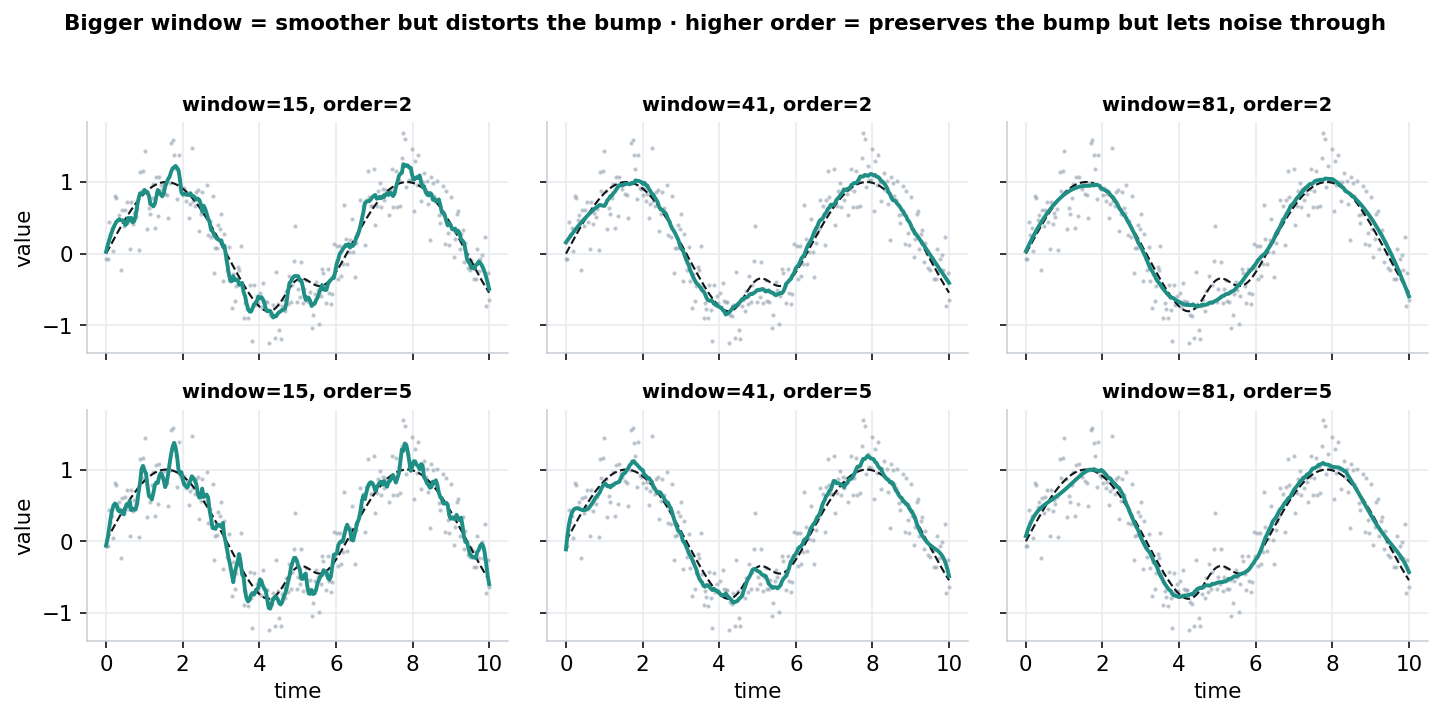
The trade-off, visualised. Across: wider windows smooth more but erase the sharp bump. Down: higher order rescues the bump but readmits noise.
A mental model that could be useful: start by picking the window from the width of the features that should be kept (it should be comfortably narrower than them, but also wider than the noise frequency we want to filter out), then pick the smallest order that preserves their shape. A cubic (order 3) is a reasonable default; orders 4–5 may be worth reaching for mainly when there are genuinely sharp features to defend.
Smoothed derivatives: the bonus feature
A feature often missed is where Savitzky-Golay starts to look like more than a nicer moving average. Differentiating noisy data is notoriously awkward: the naive approach — successive differences (np.gradient) — tends to amplify noise, because differencing emphasises exactly the high-frequency jitter we wanted gone.
Savitzky-Golay offers a way around this. Since each window is already described by a fitted polynomial, we can ask for the derivative of that polynomial instead of its value — in the same pass, with the same smoothing. In the SciPy implementation, we can pass deriv=1 (and delta, the sample spacing, so the units come out right):
dx = x[1] - x[0]

naive    = np.gradient(noisy, dx)                       # noisy mess
velocity = savgol_filter(noisy, window_length=31,
                         polyorder=3, deriv=1, delta=dx)  # much cleaner
Recovering velocity from a noisy position signal makes the difference fairly stark:
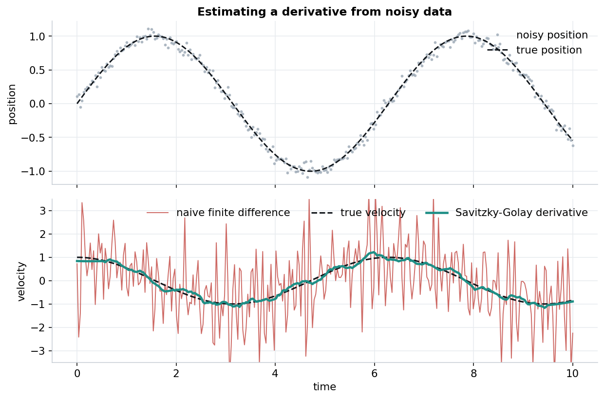
Recovering a derivative from noisy data. Naive finite differencing (red) is hard to use; the Savitzky-Golay derivative (teal) tracks the truth closely.
The red line — a finite difference of the noisy samples — is essentially unusable. The teal line — deriv=1 from the very same filter call — sits close to the true velocity. The same trick gives a smoothed second derivative (deriv=2) for curvature and inflection points. This is part of why Savitzky-Golay shows up in fields like spectroscopy and motion analysis, where differentiating real measurements matters. A plain moving average doesn’t give us this directly.
Same filter, Go implementation
The technique still travels, when not in Python. The Go package pconstantinou/savitzkygolay implements the same filter, taking the data and the corresponding x-positions:
package main

import (
	"fmt"

	sg "github.com/pconstantinou/savitzkygolay"
)

func main() {
	ys := loadYourNoisySamples() // []float64 of measurements
	xs := make([]float64, len(ys))
	for i := range xs {
		xs[i] = float64(i)
	}

	// 3rd-order polynomial over an 11-point window (NewFilterWindow default),
	// or NewFilter(window, derivative, polynomial) for full control.
	filter, err := sg.NewFilterWindow(11)
	if err != nil {
		panic(err)
	}

	smooth, err := filter.Process(ys, xs)
	if err != nil {
		panic(err)
	}
	fmt.Println(smooth)
}
The constructor precomputes the weights (cost grows with the square of the window size), and the Filter can be reused across many series to amortise that. NewFilter(window, derivative, polynomial) exposes the derivative order, so the smoothed-derivative trick from above is available here too.
What about lag?
Savitzky-Golay is often sold as the filter “without lag.” This is conditionally true and stated too casually it can mislead — so it is worth being precise, because lag is a real and useful idea.
Lag is mostly a property of causal filtering, not of averaging in general. A trailing (causal) moving average — the mean of the last N points, the kind common in finance — lags by roughly half its window, because its output at time t really describes the data centred at t − N/2. A centred moving average, which uses as many points ahead as behind, has essentially zero phase delay. So does Savitzky-Golay. Here are all three on the same noisy bump:
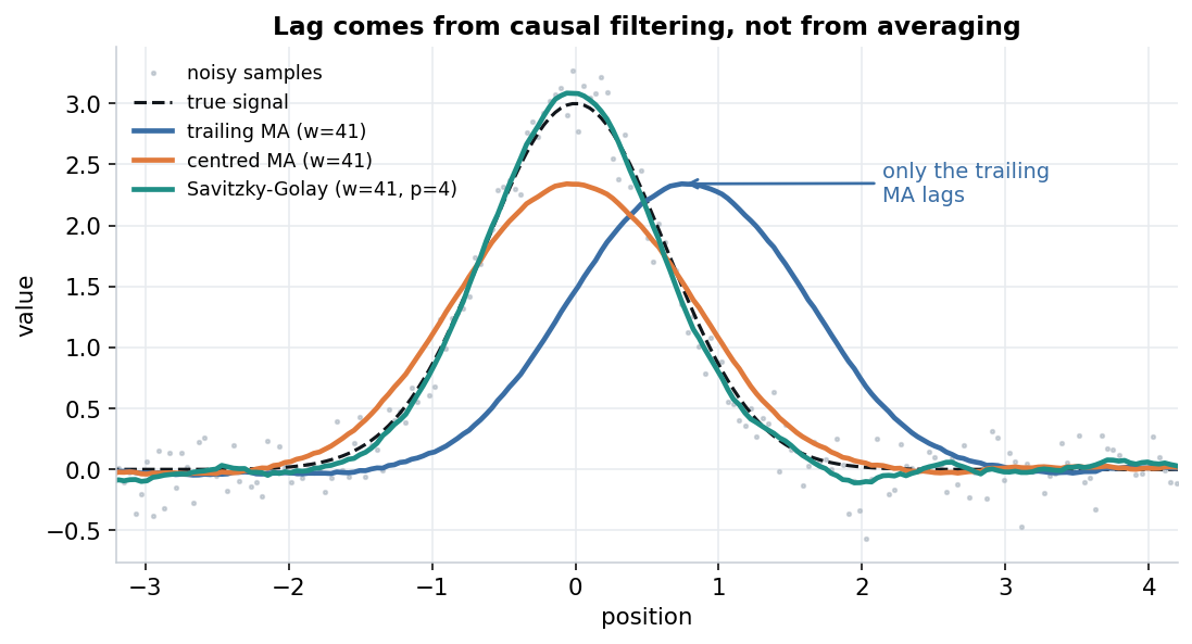
Only the trailing average lags. The centred average and Savitzky-Golay sit at roughly the right position — the centred average just flattens the peak, while SG keeps more of it.
On this bump the trailing average’s peak lands about half a window late; the centred average and SG land within a sample of the truth. Two honest conclusions follow:
- On historical data, lag is largely moot. We have the whole series, so we can centre every filter, and none of them really lag. The meaningful difference between a centred moving average and Savitzky-Golay is the one from the first figure — shape, not timing.
- On a live signal, Savitzky-Golay doesn’t rescue us from lag. The zero-lag behaviour relies on a symmetric window — points from both sides of the centre. The latest sample of a stream has no future points yet, so a centred Savitzky-Golay estimate for it only settles once enough later samples arrive: a delay of about half a window, much like the trailing average. Causal SG variants exist, but they trade some accuracy for immediacy.
So we’d reach for Savitzky-Golay mainly for shape preservation and clean derivatives, rather than for any special immunity to lag.
Derivatives: rate of change, swings, and volatility
These derivative tricks aren’t tied to any one field, but they line up neatly with questions that come up a lot in markets — where the moving average and its exponential cousin, the EMA, are the usual smoothers. So let’s borrow a market-flavoured example and put the first (and second) derivative to work on a synthetic, price-like series. Everything below is illustrative, on made-up data.
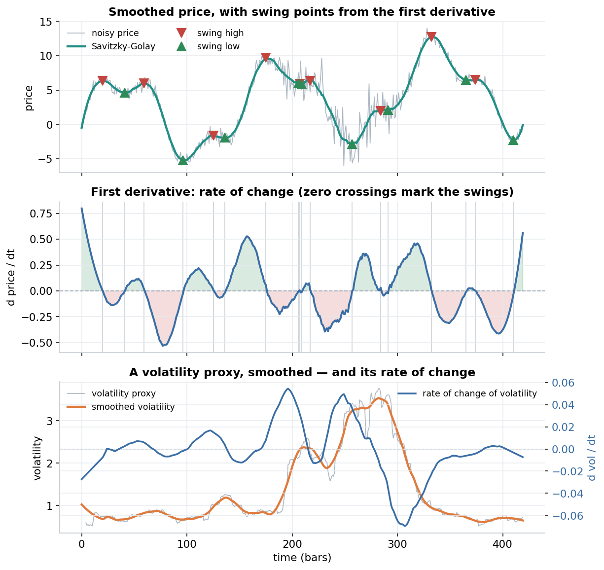
One savgol_filter call, three readings: smoothed price with swing points (top), the first derivative as a rate of change (middle), and the same idea on a volatility proxy (bottom). Synthetic data, for illustration.
A few things fall out of the same call:
- Swings (top). A swing high is just a point where the smoothed slope flips from positive to negative, and a swing low the reverse — that is, where the first derivative changes sign. Marking those zero-crossings tends to give steadier turning points than hunting for local maxima on the raw, noisy price. In the choppier middle stretch a few extra swings appear; how many we get is governed by the same two knobs as before.
- Rate of change (middle). The first derivative is a smoothed rate of change — the slope, or “velocity”, of price. Its sign tells us which leg we’re on (rising versus falling) and its magnitude how fast. The second derivative (
deriv=2) adds curvature, or “acceleration”: when it flips sign the slope has stopped steepening and begun to roll over, which can hint a swing is forming a little before the price itself confirms it. - Rate of change of volatility (bottom). The same recipe works on a volatility proxy. We take a noisy rolling-volatility estimate, smooth it, and read off its first derivative — a gentle sense of whether volatility is building or calming, rather than just its level.
It’s the kind of smoothed, derivative-based monitoring that the usual MA/EMA toolkit doesn’t hand us directly. How sensitive the swings and rates are is set by the same window and order from earlier: a wider window or lower order gives fewer, slower readings; a narrower window or higher order picks up finer moves (and more noise). None of this should be taken as a trading rule or advice, it’s just a demonstration of information extraction from noisy data, such as price and volatility.
The catch on live data
There’s an important caveat the finance world names well. Because a centred Savitzky-Golay looks both ways, its most recent values keep shifting as new bars arrive — traders call this “repainting,” and it’s the very same symmetric-window, non-causal property we met under lag (see the TradingView SG indicator discussions, or this quant write-up, which notes the recent estimates can track the latest price too closely). Two consequences worth keeping in mind:
- A centred SG used in a backtest can quietly leak the future: treating its values as if they were known at the time is look-ahead bias, which tends to flatter results. For decisions that must act on the latest bar, causal tools — an EMA, or a Kalman filter — are usually a safer default; Savitzky-Golay and LOESS sit more comfortably in retrospective analysis where shape is what we’re after.
- The deeper split isn’t SMA vs EMA vs Savitzky-Golay, but causal vs centred: an EMA estimates the level now from the past, while a centred SG estimates a value inside the series using both sides. Different questions, so they aren’t quite interchangeable.
Used with that in mind — for study and post-hoc analysis rather than live signals — Savitzky-Golay and its derivatives are a useful addition to the smoothing toolkit.
When we’d reach for something else
No filter is free. We’d skip Savitzky-Golay, or use it carefully, when:
- The signal has genuine steps or discontinuities. A polynomial fit can “ring” around a sharp edge (Gibbs-like overshoot). For piecewise-constant data, a median filter is often the better tool.
- The order is too high for the window. Push the order up and the fit starts following the noise — overfitting, the same trap as anywhere else. The param-sweep above shows the symptom.
- We need the freshest sample of a live stream. As above, the centred window costs about half a window of latency. We have to either budget for it, or use a causal variant and accept some accuracy loss.
Edges deserve care too: the standard implementation fits a polynomial to the final partial windows to fill in the boundaries (SciPy’s mode parameter), which is reasonable but generally a little less trustworthy than the interior.
Takeaways
- A moving average doesn’t only remove noise — it tends to soften structure, flattening peaks and smearing shapes. Even a centred one, with no lag at all, pulled our peak down by about 30%.
- Savitzky-Golay swaps “average the window” for “fit a small polynomial to the window,” which is curvature-aware and keeps more of the shape, while still being just one convolution.
- Two tunable parameters: window (from the width of the features to keep) and order (smallest that preserves their shape; 3 is a fine starting point).
- A standout is clean derivatives from noisy data — something a plain moving average doesn’t readily deliver.
- Depending on the field of application, lag may be unavoidable. On a live stream Savitzky-Golay lags about as much as a trailing average — what traders call “repainting.”
- We’d pick it for shape preservation and derivatives, and lean on causal tools when the latest point has to be right.
Next time we type rolling().mean() out of habit, it is worth asking whether we actually need the signal’s shape preserved. If we do, Savitzky-Golay is worth a look.
Enjoy coding!